Monitoring the Solar Wind
The following is presented for those who would like an introduction to the solar wind and how it is monitored.
1 Solar Wind Measurements
Before any spacecraft had flown, in the 19th and early 20th Centuries, people hypothesized through deduction and the observation of phenomena like sunspots, solar flares, geomagnetic disturbances, comet tails, and auroras that there was a continuous flux of solar particles expanding away from the Sun. At the dawn of the space age, in the 1950’s, work by physicists such as L. Biermann, S. Chapman, and E. N. Parker lead to advances in the theory of the outflow of matter from the Sun. Biermann pointed out that the observed motions of comet tails indicate that gas streams outward from the sun, radially, with speeds ranging from 500 to 1500 km/s. Chapman theorized that a static atmosphere of the sun extended far beyond the Earth’s orbit. Parker predicted that the Sun’s corona could not remain in static equilibrium but had to be continually expanding since the interstellar pressure could not contain a static corona. He termed this outflow from the Sun the "solar wind”. He predicted that the solar wind was directed radially from the Sun with a supersonic flow of hundreds of km per second. However, there was strong opposition to Parker’s solar wind theory. It took evidence from satellites to prove that there was a solar wind, as Parker theorized.
Soviet spacecraft equipped with “ion traps” (Konstantin Gringauz’s gridded Faraday cups) were the first to sample the solar wind. Lunik II (launched in 1959) measured a positive ion flux of ~2x108 cm-2 s-1. Lunik II did not measure the direction of the flux and could only determine that the flux was for particles with energy greater than 15 eV. The Lunik II measurements lent validity to Parker’s solar wind theory that had just been published in 1958.
In the three years after Lunik II launched, a number of improved instruments designed to analyze the solar wind either failed to launch or failed to detect the wind. Those that failed to detect the wind either pointed in the wrong direction or were ‘blinded’ by sunlight when they did point in the right direction. One instrument that worked was MIT’s ion trap on NASA's Explorer 10. It was designed to explore the nightside tail of the magnetosphere but was often immersed in the solar wind.
In 1962 a curved plate ion energy analyzer equipped with a faraday cup particle detector was launched as part of the payload of Mariner 2. Mariner 2 returned an ion energy spectrum of the solar wind almost continuously for 113 days. An example of the data collected by Mariner 2 is shown below.
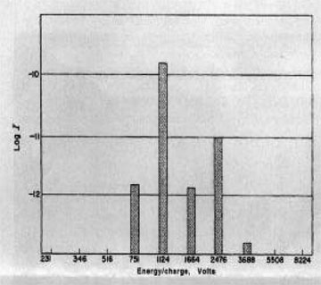
Mariner 2 spectra contained only one to five energy/charge channels of between 231-8224 eV/q. Mariner 2 data showed that the solar wind blew continuously within the instrument’s field of view, which could not look farther than 10˚ from the sun. The spectra showed that the wind varied in speed from 400 to 700 km/sec. Researchers learned that the solar wind was organized into high- and low-speed streams, that the streams had steepened leading edges with higher densities due to pileup, and that the proton temperature varied directly with the speed. Five data point spectra showed that alpha particles had the same thermal speeds and bulk speeds as protons and showed that the ratio of alphas to protons was highly variable. It is clear that by 1962 space-borne ion energy analyzers were proving valuable in monitoring the solar wind. Correlations were made between solar wind speed as measured by Mariner 2 and geomagnetic activity as measured at stations on the Earth. Thus, there was direct evidence of the connection between solar wind conditions (solar wind speed) and effects felt on the Earth’s surface (geomagnetic field fluctuations).
2 Improved Solar Wind Measurements
The solar wind consists of positively and negatively charged particles in about equal numbers so that the bulk charge is about zero (a plasma). Even though ions can be either positively charged or negatively charged, when solar wind scientists speak of ‘ions’ they mean positively charged particles. The use of the term ‘ion’ to denote exclusively ions with a positive charge is peculiar to field of solar wind science. In chemistry, to avoid confusion, positively charged ions are denoted ‘cations’ and negatively charged ions are denoted ‘anions’. Throughout this document I will adhere to the convention used in solar wind science: ‘ions’ are cations. The vast majority of solar wind ions are protons (the hydrogen atom with the electron removed, H+). The solar wind composition is also about 4% alpha particles (He++) by number. But since He has a mass 4 times H, the solar wind is about 16% alphas by mass. The negatively charged particles that balance out the charge in the solar wind plasma are almost exclusively electrons.
Instruments designed to monitor the solar wind usually return data in terms of particle abundance versus particle energy. For instruments that make a current measurement to determine the flux of particles the plots of the raw data collected (spectra) are usually of ‘current vs. energy’ and for instruments that are able to count particles the plots are usually ‘counts vs. energy’.
Below is a spectrum collected by the electrostatic analyzer (ESA) curved plate analyzer (CPA) that was launched on the ESRO HEOS-1 satellite in 1968. The ‘hemispherical analyzer’ consisted of a hemispherical electrostatic deflector and a Faraday cup detector that was able to measure the current from ions admitted in 28 adjacent energy channels from about 200 to about 1600 eV/q. The sensitivity of the instrument was approximately 107 cm-2 s-1 for protons and 5x106 cm-2 s-1 for alphas. A complete spectrum along the entire energy range was taken in 6.4 minutes.
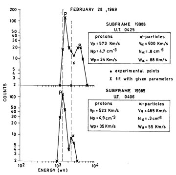
The spectrum is more detailed than the spectra collected by Mariner 2. To the right of the ‘counts vs. energy’ plot is the derived velocity ‘V’, density ‘N’, and temperature ‘W’ for both protons (denoted with a subscript ‘p’) and alpha particles (denoted with a subscript ‘α’). It is clear that by 1968 better quality spectra were being collected so that characteristics such as speed, density and temperature for the major components of the solar wind could be derived.
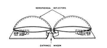
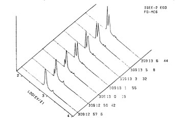
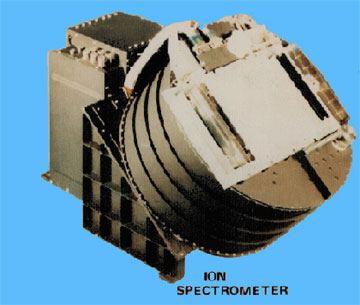
In 1977 the ISEE-2 spacecraft was launched. It also contained a hemispherical analyzer for collecting spectra of the solar wind. The spectrometer, shown below, was improved over the HEOS-1 spectrometer in that it contained channel electron multipiers (CEMs) rather than Faraday cup particle sensors. It also had an energy resolution of 4% ΔE/E, which likely compares favorably to instruments that were flown before it was, and, in fact, compares favorably to instruments that are now flown. The device was able to detect particles at three orders of magnitude lower fluxes (104 cm-2 s-1) than the HEOS-1 instrument. The remarkable increase in sensitivity is not surprising considering the that CEMs are capable of producing a count for each particle that strikes them and Faraday cups must be struck by a large enough flux of charged particles that a net current can be measured.
The dual-hemisphere CEM equipped ISEE-2 instrument and spectra from the instrument are shown below:
Jumping forward two decades, the SWEPAM-I instrument on the ACE spacecraft was launched in 1997 and is currently collecting spectra of the solar wind ions. For a given spectrum, SWEPAM-I collects data at 40 energies selected from a set of 200 possible energies (at energies between 260 eV and 36,000 eV with 5% ΔE/E instrumental energy resolution). Below are two spectra from SWEPAM-I, one for a typical high speed, low density solar wind and the other for a typical low speed high density solar wind, as will be described later.
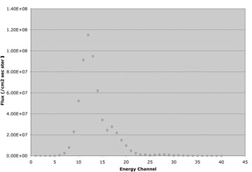
First, a typical high speed, low density differential directional number flux spectrum from SWEPAM-I:
Second, a typical low speed, high density differential directional number flux spectrum from SWEPAM-I:
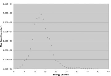
The plots shown above differ from the plots of raw data from Mariner 2, ESRO HEOS-1, and ISEE-2 in that the particle flux at each energy is given in units of flux rather than counts. The ‘differential directional number flux’ units of counts cm-2 s-1 are useful for estimating the performance of instruments that have not yet retrieved data in the solar wind. The spectra from SWEPAM-I are analyzed in real-time for solar wind properties such as velocity, temperature, and density.
3 Interpreting Solar Wind Ion Energy Spectra
The speed, temperature, and density of the solar wind are derived from the ion energy spectra that are collected by satellites. Below is a graphical representation of a solar wind spectrum (this is a spectrum from SWEPAM-I).

The solar wind speed for protons is derived from proton peak energy (the channel with the most counts per second) converted from kinetic energy to speed by the formula; 10-3 x [(proton peak location in eV) x 1.8 x 10⁸]1/2= proton speed in km/s. The solar wind speed can be as slow as 260 km/s and faster than 750 km/s, but are typically about 400 km/s. A similar determination is made for alphas by determining the peak energy for alphas and considering the four-fold greater mass of alpha particles. A ‘double Maxwellian’ curve fit of the data, such as is done with data gathered by WIND, can be used to better determine the two peak locations.
Doppler broadening of the proton and alpha peaks indicate the solar wind temperature. By measuring the ‘half-width at half maximum’ of each peak, the temperature can be determined from the appropriate formula.
The density of the solar wind is simply the ‘particles per cubic centimeter’ integrated over all energies in the peak. A formula is used, after the double Maxwellian curve fit, to translate counts per second to particles/cm3. The solar wind density is also derived from the spectrum. Its density can vary between 0.1/cm3 and 100/cm3.
In addition to varying in its speed, temperature, and density, the solar wind varies in it’s angular ‘size’ and direction of flow. Although the solar wind is almost always directed within +/-10 degrees of radially from the sun (as was discovered by Mariner 2), it has been reported to vary by more than 10 degrees from radially at times. Additionally, the radial wind is “aberrated” to 5˚ (or 4˚ is also reported) due to the an L1 spacecraft’s orbital motion (a speed of about 30 km/s) around the sun. Therefore, when the solar wind flows in a purely radial direction from the sun, it appears to be coming slightly from the west when observed from a spacecraft sharing the earth’s orbital motion. The beam also has a non-zero solid angle cross section that varies in shape; sometimes narrow, sometimes wide, sometimes circular, sometimes elliptical. As a result of the solar wind ‘beam’ divergence, it is not unusual to see solar wind ion spectral counts in seven (5˚ x 5˚) SWEPAM-I sectors.
4 Solar Wind Monitors Today
Two solar wind monitors will be described. The SWEPAM-I instrument on the ACE spacecraft and the Faraday Cup (FC) on the WIND spacecraft. Both instruments return spectra that are used to determine solar wind speed, temperature, density, and direction and report them on a day-to-day basis.
SWEPAM-I is spun and has 16 channel electron multiplier detectors that look at 16 slightly different directions simultaneously so that it can make a full 3-D plasma measurement of protons and alphas over 40 energy levels every 64 seconds. A photograph of the 3.7 kg SWEPAM-I instrument of the ACE spacecraft is shown below.
Each of SWEPAM-I’s 16 channels has a geometric factor of 1 to 20 x 106 cm2 sr eV/eV. ‘Geometric factor’ can be used as a gauge to compare charged particle spectrometers to each other: geometric factor is proportional to the speed at which a charged particle spectrometer can collect a spectrum when pointing at a particle beam with a given flux. Ambient particle flux and spectrometer geometric factor are important factors to consider when estimating performance characteristics such as speed and accuracy in solar wind velocity, temperature, and density determinations. Examples of solar wind spectra from SWEPAM-I have already been shown.
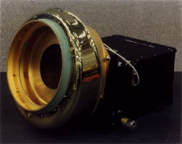
The Faraday Cup (FC) instrument on WIND is a different type of energy analyzer. Rather than filter out the desired energy particles by having them follow curved trajectories through an electric field in a curved space, the faraday cup instrument uses a ‘retarding potential’ supplied by a wire grid in front of a conducting plate.
Below is a photograph of the 5 kg Faraday Cup (FC) instrument of the WIND spacecraft.
The spectrum shown below is of the solar wind as gathered by the WIND FC instrument.
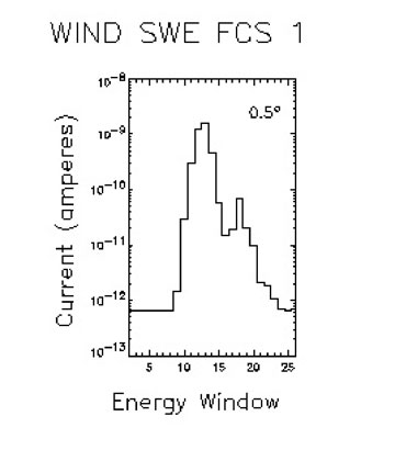
Retarding potential analyzers like the FC instrument have been flown in space to sample the solar wind from many spacecraft. Advantages of retarding potential analyzers have been reported as: compact design, large geometric factor, and the ability to retain calibration over space mission lifetimes.
5 The Goembel Instruments Solar Wind Monitor
Use of the Goembel Instruments patented curved aperture/colimator design and another proprietary Goembel Instruments technology would enable the rapid collection of spectra far superior to those now collected by SWEEPAM-I and WIND FC. Such spectra would enable unprecedented monitoring of the solar wind for speed, temperature, and density in both protons and alphas. The Goembel Instruments Solar Wind Monitor offers at least an order of magnitude better performance and would require fewer spacecraft resources (mass and power) than either SWEEPAM-I or WIND FC.